4. AC circuits

For the analyzes of alternating current or AC circuits the use of complex numbers is quite convenient. For the most important properties of complex numbers refer to Appendix D: Complex numbers.

Complex notation signals

Symbols

A sinusoidal signal is completely characterized by its amplitude, frequency and phase. If such a signal is fed through an electronic circuit in many cases the amplitude and the phase will change, while the frequency remains the same. The amplitude \(\hat{x}\) and the phase \(\varphi\) of the sinusoidal signal \(x(t)=\hat{x} \cos (\omega t+\varphi)\) are very similar to the modulus and the argument of a complex number. A complex number \(X=|X|\exp^{j(\omega t+\varphi)}\) is shown in a complex plane as a rotating vector of length \(|X|\) and an angular frequency \(\omega\). When \( t=\pm nT \), the argument of \(X\) is exactly equal to \( \varphi \). Therefore \(|X|\) is equivalent to the amplitude \(\hat{x}\) of the signal, and the argument of \(X\) is equivalent to the phase factor \(\varphi\) of the signal. Furthermore, the real part of \(X\) is equal to the function \(x(t)\).

Complex impedances

For a resistor Ohm’s law \( R=\frac{V}{I} \) applies. This relationship applies to both DC and AC signals. For AC signals the current through, and the voltage across a resistor is in phase with each other.
For a capacitor and a coil, however, this is not the case.
Let us assume that the voltage across a capacitor is given by \( v(t)=\hat{v} \sin \omega t \), then it follows that the current is given by:

(30)\[\begin{split} \left. \begin{align} v(t) & = \hat{v} \sin (\omega t) \\ i &= C\dfrac{dv}{dt} \end{align} \right\} \Rightarrow i(t) = \omega C \hat{v} \cos (\omega t) \end{split}\]

Thus, the current runs \(90 ^{\rm o}\) in phase before the voltage. Naively applying Ohm’s law provides a remarkable result for the resistance of a capacitor:

(31)\[ R_{c}=\dfrac{v(t)}{i(t)}=\dfrac{v \sin (\omega t)}{\omega C \hat{v} \cos (\omega t)}=\dfrac{1}{\omega C} \tan (\omega t) \]

This quantity ranges from \( -\infty \) to \( +\infty \). That is certainly not a useful quantity. That in itself is not surprising, because of the attempt to describe two things with one variable: the relationship between the magnitude of the voltage and current on the one hand, and the phase difference between voltage and current on the other.

Complex numbers are handy, as they show both the magnitude and the phase of a variable. Therefore for AC signals we switch to a complex resistance, or impedance \(Z\). This defines the ratio of the complex voltage \(V\) and the complex current \(I\):

(32)\[ \nonumber Z=\dfrac{V}{I} \]

(33)\[ |Z|=\dfrac{|V|}{|I|} \]

(45)\[ \nonumber \arg Z=\arg V-\arg I \]

Thus \(\arg Z\) indicates to what extent the voltage phase is ahead of the current.
For the impedance of a capacitor holds:

(35)\[\begin{split} \left.\begin{align} V &= \hat{v}\exp^{j\omega t} \\ I &= C\dfrac{dV}{dt} = j\omega C\hat{v}\exp^{j\omega t} \end{align} \right\} \Rightarrow Z_{c} = \dfrac{1}{j\omega C} \end{split}\]

Using eqn. (184) eqn.(35) may be written as:

(36)\[\begin{split} \begin{split} |Z| &=\dfrac{1}{\omega C} \\ \arg Z &= 0 - \tan^{-1} \left (\dfrac{\omega C}{0}\right )= -\dfrac{\pi}{2} \end{split} \end{split}\]

From eqn.(36) it follows that the voltage lags \(90 ^{\rm o}\) in phase with the current.
Similarly for a coil with inductance \(L\), where \(V=\frac{LdI}{dt}\), the impedance is given by:

(37)\[ Z_{L}=j\omega L \]

The impedance of a resistor is real, since there is no phase difference between the current through, and the voltage across a resistor:

(38)\[ Z_{R}=R \]

For impedances in series or in parallel, the same calculation rules apply as for ordinary resistors.

• For impedances \(Z_1\), \(Z_2\), \(Z_3\), …. in series eqn.(39) applies:

(39)\[ Z=Z_{1}+Z_{2}+Z_{3}+ .... \]

• For impedances \(Z_1\), \(Z_2\), \(Z_3\), …. in parallel eqn. (40) applies:

(40)\[ \dfrac{1}{Z}=\dfrac{1}{Z_{1}}+\dfrac{1}{Z_{2}}+\dfrac{1}{Z_{3}}+ .... \]

Complex input and output impedance

The theorem of Thévenin and superposition theorem, as discussed in Thévenin’s theorem and Superposition theorem, are also applicable if there are impedances, instead of resistors. In fact, it comes down to replacing the word resistance by impedance in the theorems.
On the basis of the theorem of Thévenin a signal generator can for example be represented by the circuit shown in Fig. 40. \( Z_{u} \) is the output impedance or source impedance.

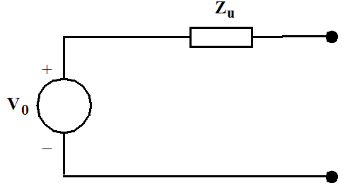
Fig. 40 Signal generator according Thévenin

For a correct signal transmission not only the output impedance of the generator plays a part, but also the input impedance of the circuit to which the generator is connected.

Complex transfer function \(A(\omega)\)

The function which describes the relationship between the output and input signal of a circuit, as indicated in Transfer function, is known as the transfer function. In general this function will be frequency dependent:

Attention

In many electronic books the term frequency is used when angle frequency is actually meant. Also in this syllabus this is repeatedly done. Usually the equations make it clear whether \(f\) or \(\omega\) is meant. Because \( f=\omega/2\pi\) the difference in the calculations is a factor of \(2\pi\).

Because there is often a frequency-dependent phase shift between the output and input signal, the description will tend to be a complex function. The transfer function is therefore divided into two functions, the amplitude function and the phase function. The amplitude function indicates the ratio between the amplitude output and input signals as a function of the frequency, and is equal to the modulus of the transfer function \(|A|\). The phase function gives the phase difference between the output and input signal, and is equal to \(\arg(A) \).

Note

Please note that when calculating the phase function the function \(\tan^{-1}\) is used for the calculation, which is defined only to the interval \(-\frac{\pi}{2}\) to \(+\frac{\pi}{2}\). To keep the phase function continuously, the function needs to be added in some cases with a whole number of times \(\pi\). See also Appendix D.

Bode plot

The usual way to visualize the frequency dependence of the transfer function is to draw a frequency diagram, in which both the amplitude function and the phase function is plotted against the frequency. These two graphs together are called the Bode plot (see Fig. 41).

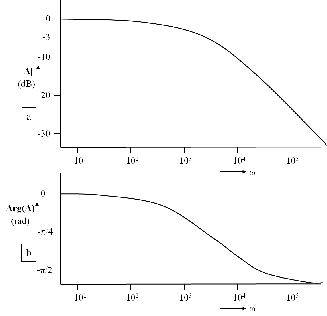
Fig. 41 Bode plot: (a) amplitude; (b) phase transfer

The frequency axis has a logarithmic scale as well as the axis for the amplitude function (unit decibel), while the scale for the phase function is linear (unit degrees or radians).
Two key terms in frequency analysis systems are the octave and the decade. An octave is the doubling or halving of the frequency, while the decade is the change in frequency by a factor of 10. In the following sections, a number of filter circuits are discussed.

First order filter

In Fig. 42 the schematic of a circuit is shown, which passes low frequencies and filters out high frequencies. This circuit is known as a low-pass filter.

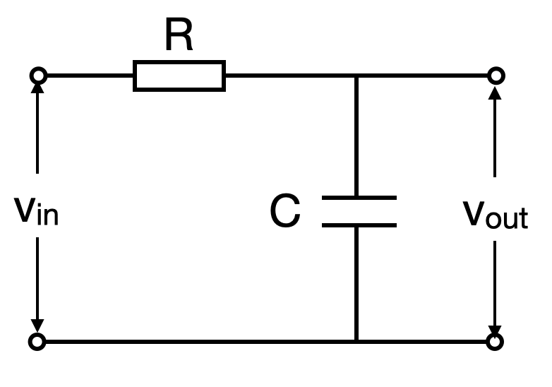
Fig. 42 Low-pass filter

The transfer function of the low-pass filter (see Fig. 42) is given by:

(41)\[ A(\omega)=\dfrac{1/(j\omega C)}{1/(j\omega C) + R}=\dfrac{1}{1+j\omega CR} \]

The power of \(\omega\) determines the order of the filter. This is therefore a first order filter. The amplitude function is given by:

(42)\[ |A(\omega)|=\dfrac{1}{\sqrt{1+(\omega CR)^{2}}}. \]

An important quantity is the 3 dB point. This is the frequency at which the output signal is 3 dB or a factor \( \sqrt{2} \) (see appendix C) lower than the maximum output signal. This frequency is also referred to as the cut-off frequency. For the -3 dB point:

(43)\[ \dfrac{|A_{3 \, {\rm dB}}|}{|A_{\rm max}|}=\dfrac{1}{2}\sqrt{2}=0.707. \]

For the low-pass filter it follows from the eqns.(42) and (43) that \(\omega_{3 \, {\rm dB}} = 1/RC\) (check this!).
The product \(RC\), which has the dimension of time, is known as the \(RC\) time of the filter. This time is often indicated by \( \tau \). Hence, \( \omega_{3 \, {\rm dB}}=1/\tau \)

The phase difference between output and input signal is given by:

(44)\[ \varphi = \tan^{-1} \dfrac{0}{1} - \tan^{-1} \dfrac{\omega R C}{1} = - \tan^{-1} (\omega R C). \]

For \(\omega = \omega_{3 \, {\rm dB}}\) \(\tan \varphi=-1 \Rightarrow \varphi=-45^{o} \).

In Fig. 43 the Bode plot is shown for a low-pass filter.

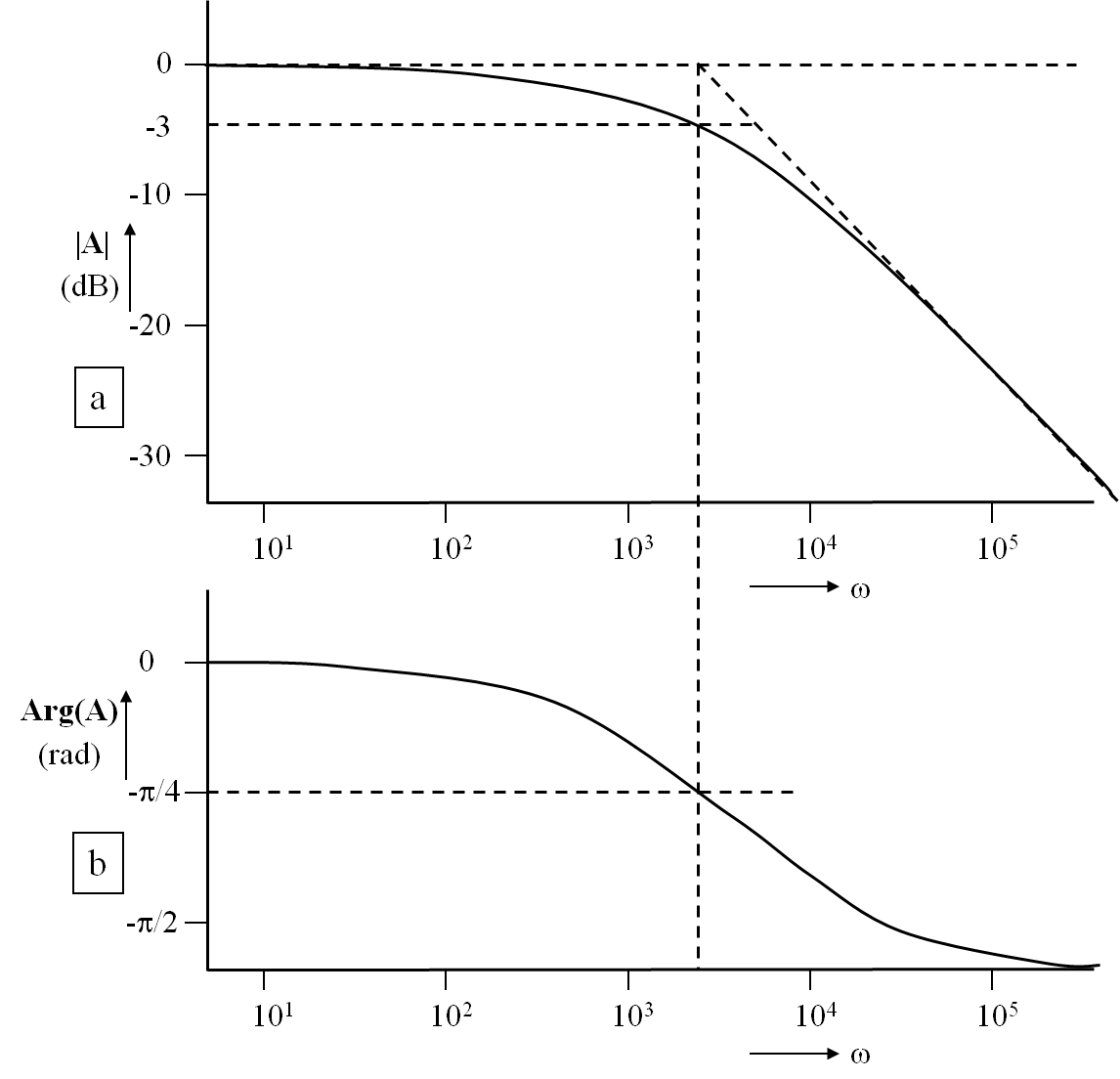
Fig. 43 Bode plot low-pass filter

In many cases it is not necessary to know the exact behaviour of the transfer functions, and is it sufficient to know the asymptotic behaviour.

Table 1 Asymptotic behaviour low-pass filter

\(\omega\ll\dfrac{1}{\tau}\)	\(\mid A \mid \; \approx1\)	\(\phi\approx0\)
\(\omega=\dfrac{1}{\tau}\)	\(\mid A \mid \; =\dfrac{1}{2}\sqrt{2}\)	\(\phi=-\dfrac{\pi}{4}\)
\(\omega\gg\dfrac{1}{\tau}\)	\(\mid A \mid \; \approx\dfrac{1}{\omega\tau}\)	\(\phi\approx-\dfrac{\pi}{2}\)

For low frequencies the signal is hardly attenuated. For high frequencies, the signal drops proportional with \( \omega \). Doubling of the frequency (octave) means that the output signal is halved. In decibel notation this means 6 dB/octave or -20 dB/decade.
From tab1 it can be seen that the phase of the output signal is lagging behind the phase of the input signal. One speaks in this case of phase-lag. If the signal is leading it is phase-lead.

Exercise 4.1

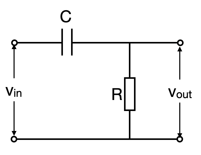
Fig. 44 High-pass filter

• Determine the complex transfer, amplitude and phase functions of this filter.

• Determine the cut-off frequency as a function of R and C.

• Investigate the asymptotic behaviour of this filter.

• Is there a phase-lag or phase-lead in this filter

• Verify your results with the use of Multisim. Make use of the Bode plotter.
  Amplitude and phase functions can be shown with the “grapher” (below in the View-menu of Multisim). In Multisim the data of the selected graph can be stored with the menu item “Export to Excel” or under Tools menu.

Answer

The transfer function is given by (voltage divider)

(45)\[ A ( \omega ) = \frac{V_{\rm out}}{V_{\rm in}} = \frac{R}{R + 1 / j \omega R C} = \frac{j \omega R C}{j \omega R C + 1}. \]

The amplitude is given by

(46)\[ | A ( \omega ) | = \frac{| \ j \omega R C |}{| \ j \omega R C + 1 |} = \frac{\omega R C}{\sqrt{1 + ( \omega R C )^2}}. \]

The phase function is given by

(47)\[\begin{split} \begin{split} \phi &= {\rm arg} \; ( j \omega R C ) - {\rm arg} \; (j \omega R C + 1 ) \\ &= \tan^{-1} \frac{\omega R C}{0} - \tan^{-1} \frac{\omega R C}{1} \\ &= \frac{\pi}{2} - \tan^{-1} \omega R C. \end{split} \end{split}\]

The cut-off frequency is obtained from

(48)\[ \frac{| A (\omega_{3 \; {\rm dB}}|}{| A_{\rm max}|} = \frac{1}{2} \sqrt{2}. \]

Since

(49)\[ | A_{\rm max} | = | A ( \infty) | = \frac{\infty}{\sqrt{1 + \infty^2}} = 1, \]

we get

(50)\[\begin{split} \begin{split} | A (\omega_{3 \; {\rm dB}})| &= \frac{1}{2} \sqrt{2} \rightarrow \\ \frac{\omega R C}{\sqrt{1 + ( \omega R C )^2}} &= \frac{1}{2} \sqrt{2} \rightarrow \\ \frac{( \omega R C )^2}{1 + ( \omega R C )^2} &= \frac{1}{2} \rightarrow \\ 2 ( \omega R C )^2 &= 1 + ( \omega R C )^2 \rightarrow \\ ( \omega R C )^2 &= 1 \rightarrow \\ \omega &= \frac{1}{RC}. \end{split} \end{split}\]

The asymptotic behavior is shown in tab2.

Table 2 Asymptotic behavior high-pass filter

\(\omega\ll\frac{1}{\tau}\)	\(\mid A \mid \; \approx \frac{0}{1} = 0\)	\(\phi\approx \frac{\pi}{2}\)
\(\omega=\frac{1}{\tau}\)	\(\mid A \mid \; =\frac{1}{2}\sqrt{2}\)	\(\phi=\frac{\pi}{2} - \frac{\pi}{4} = \frac{\pi}{4}\)
\(\omega\gg\frac{1}{\tau}\)	\(\mid A \mid \; \approx 1\)	\(\phi\approx \frac{\pi}{2} - \frac{\pi}{2} = 0\)

The output signal is leading the input signal so there is a phase-lead.

To construct a high-pass filter with a cut-off frequency of 5 kHz, using a 1 k\(\Omega\) resistor, the capacitor required is

(51)\[\begin{split} \begin{split} \omega &= 2 \pi f = \frac{1}{RC} \; \rightarrow \\ &= 2 \pi 5 \; {\rm kHz} = \frac{1}{1 \; {\rm k}\Omega C} \; \rightarrow \\ C &= 32 \; {\rm nF}. \end{split} \end{split}\]

The Multsim circuit is shown in Fig. 45. The bode plot amplitude and phase signals are shown in Fig. 46 and confirm the behavior of the high-pass filter.

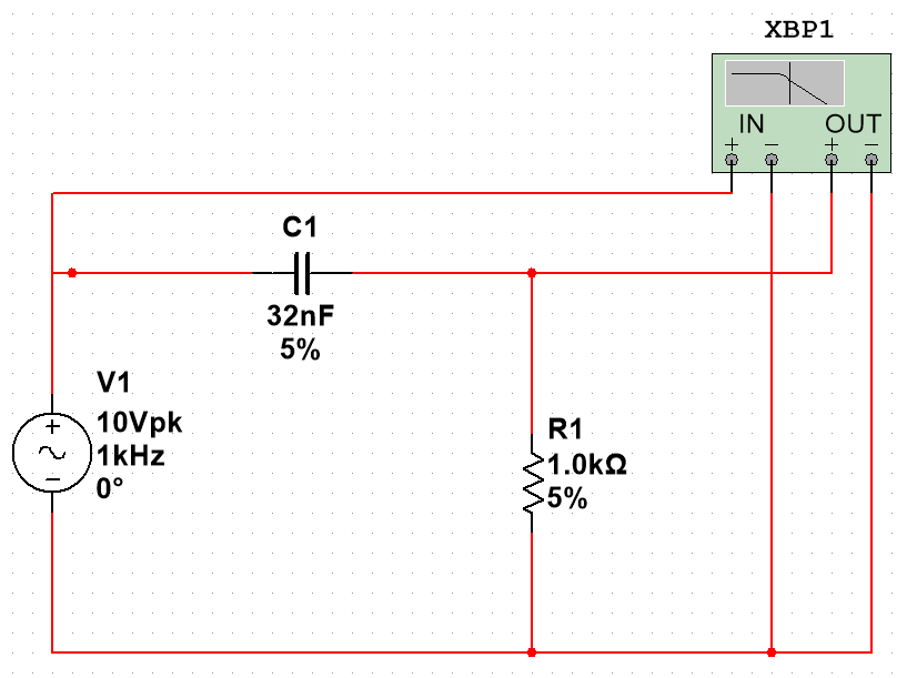
Fig. 45 High-pass filter circuit - Multisim

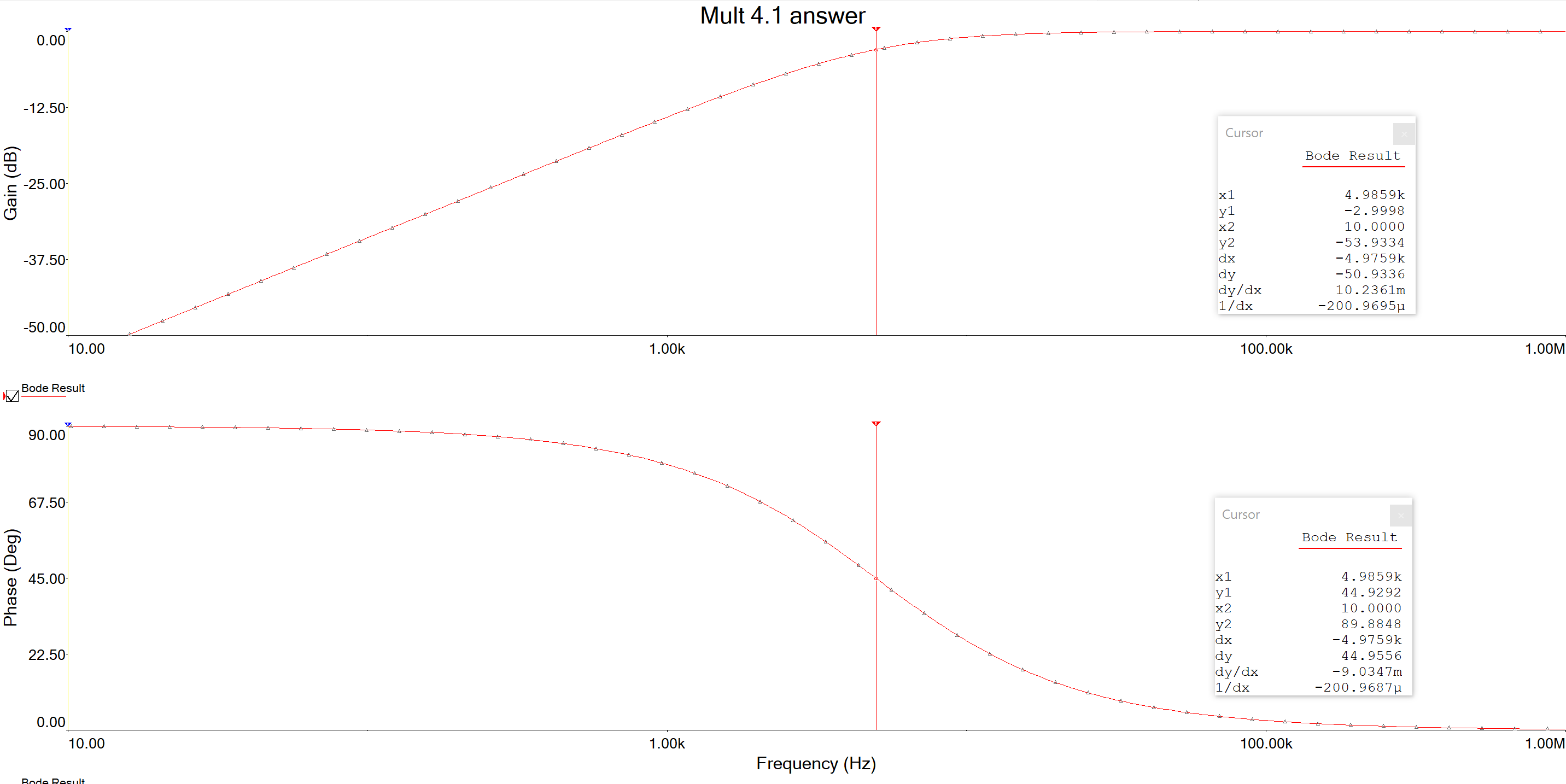
Fig. 46 Amplitude & phase Bode plot high-pass filter - Multisim results

Second order filter

An example of a second order filter is shown in Fig. 47.

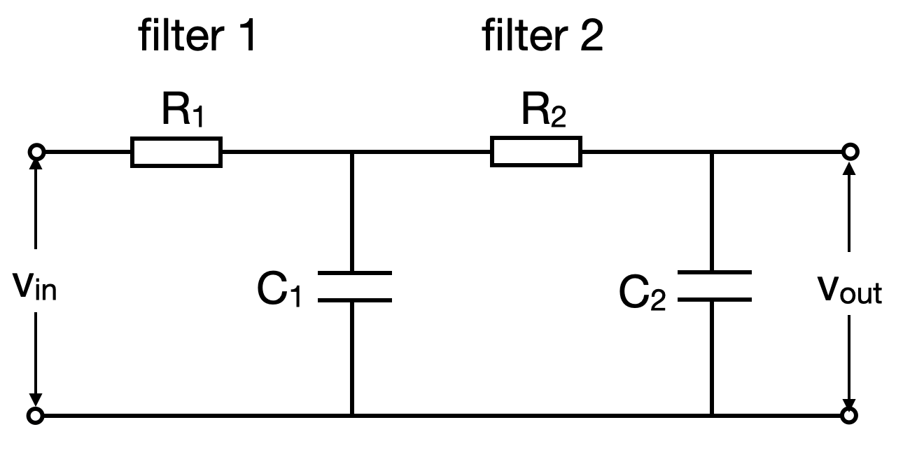
Fig. 47 Second order low-pass filter

At first it is assumed that a second filter does not influence the first. The transfer function for this circuit is then simply given by the product of the individual functions:

(52)\[\begin{split} \begin{align}\ A(\omega) & = A(\omega)_{1} \cdot A(\omega)_{2} \\ &= \left (\dfrac{1}{1+j\omega \tau}\right)^{2} \nonumber \\ & = \dfrac{1}{1+2j\omega \tau-\omega^{2}\tau^{2}}. \end{align} \end{split}\]

where \(R_{1}C_{1}=R_{2}C_{2}=\tau\).

Exercise 4.2

• Determine the amplitude and phase functions for the filter of Fig. 47.

• Investigate the asymptotic behaviour of this filter at \(1/\tau \).

• Determine how many dB/octave and how many dB/decade this filter drops for high frequencies.

• Compare your results with the data of the first order low-pass filter. If necessary show both amplitude functions in one graph.

Answer

The amplitude function of Fig. 47 is given by

(53)\[\begin{split} \begin{split} | A (\omega) | &= \frac{\ | 1 |}{| 1 + 2 j \omega \tau - \omega^2 \tau^2 |} \\ &= \frac{1}{\sqrt{(1 = \omega^2 \tau^2 )^2 + (2 \omega \tau )^2}} \\ &= \frac{1}{\sqrt{1 - 2 \omega^2 \tau^2 + \omega^4 \tau^4 + 4 \omega^2 \tau^2}} \\ &= \frac{1}{\sqrt{1 + 2 \omega^2 \tau^2 + \omega^4 \tau^4}} \\ &= \frac{1}{\sqrt{(1 + \omega^2 \tau^2)^2}} \\ &= \frac{1}{1 + \omega^2 \tau^2}. \end{split} \end{split}\]

The phase function is given by

(54)\[\begin{split} \begin{split} \phi &= {\rm arg}(1) - {\rm arg}(1 - \omega^2 \tau^2 + 2 j \omega \tau) \\ &= \tan^{-1}\frac{0}{1} - \tan^{-1} \frac{2 \omega \tau}{1 - \omega^2 \tau^2} \\ &= - \tan^{-1} \frac{2 \omega \tau}{1 - \omega^2 \tau^2} \pm k \pi. \end{split} \end{split}\]

When \(\omega \ll \frac{1}{\tau}\) the amplitude \(|A| \approx 1\) and phase \(\phi \approx 0\).
When \(\omega = \frac{1}{\tau}\) the amplitude \(|A| = \frac{1}{2}\) and phase \(\phi = - \tan^{-1} (\frac{2}{0}) = - \frac{\pi}{2}\).
When \(\omega \gg \frac{1}{\tau}\) the amplitude \(|A| \approx 0\) and phase \(\phi \approx \tan^{-1} (2 \omega \tau / - \omega^2 \tau^2) = \tan^{-1} ( 2 / - \omega \tau) \approx 0 - \pi \rightarrow - \pi\).

The amplitude and phase functions are shown in Fig. 48 and Fig. 49 for \(R_1 = R_2 = 1 \; {\rm k} \Omega\) and \(C_1 = C_2 = 32\) nF.

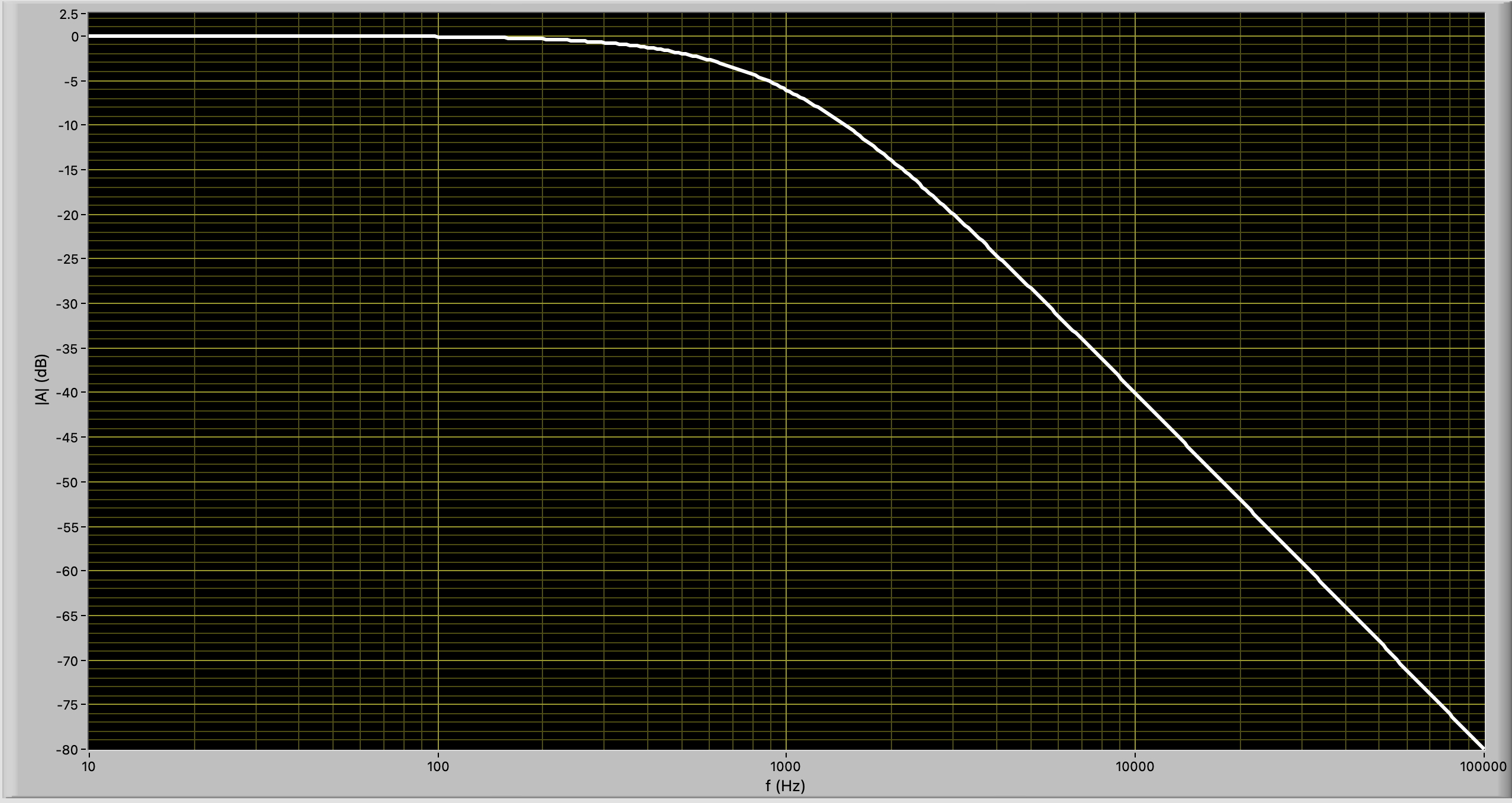
Fig. 48 Amplitude bode plot second order low-pass filter

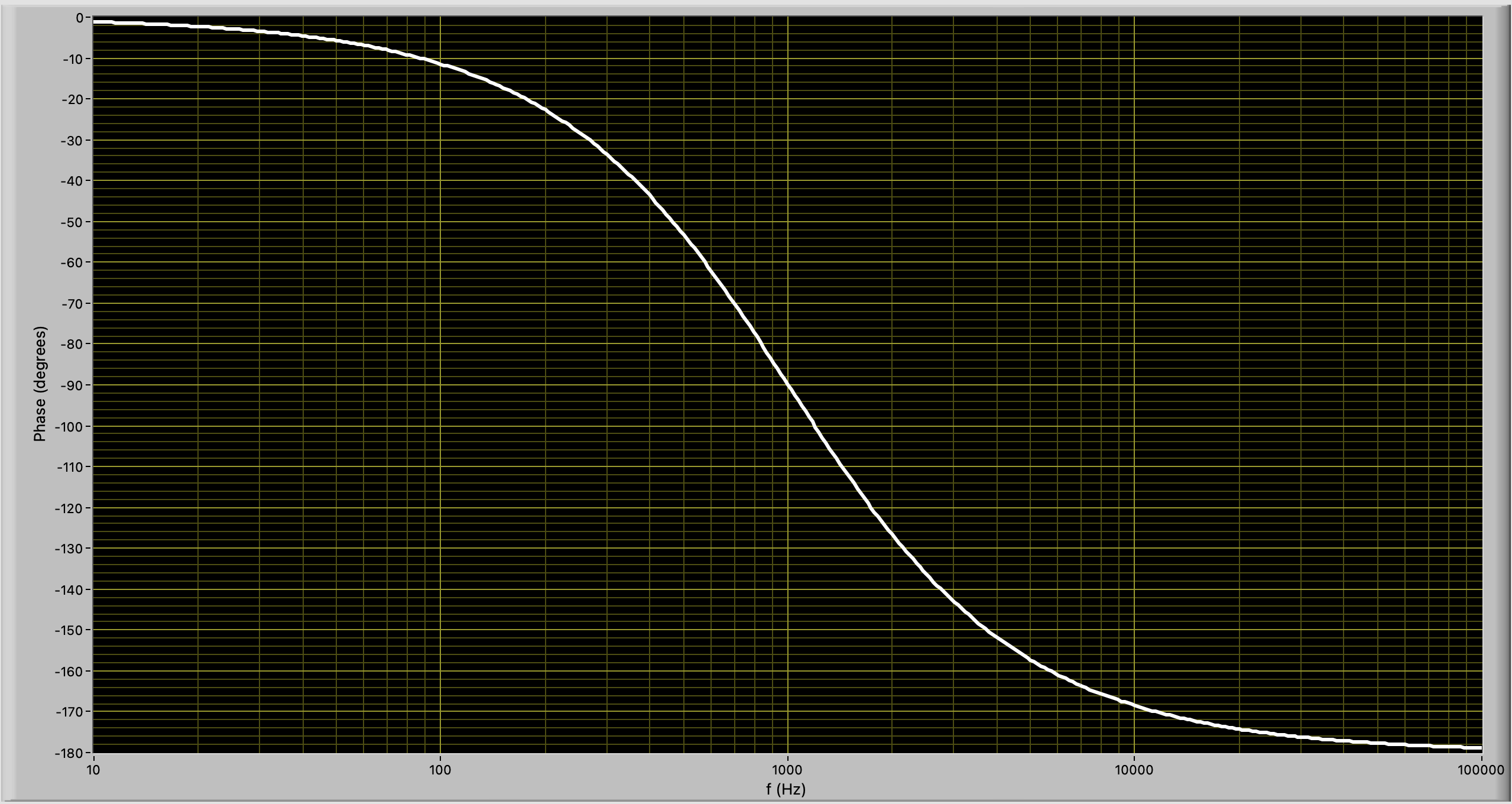
Fig. 49 Phase bode plot second order low-pass filter.

The amplitude drop for a first order LPF is -6 dB/octave and -20 dB/decade. For the second order LPF we get:

(55)\[\begin{split} \begin{split} &\omega \rightarrow 2 \omega \; {\rm gives} \; \omega^2 \rightarrow 4 \omega^2 \; {\rm so} \; 20 \log_{10} (\frac{1}{4}) =-12 \; {\rm dB}, \\ &\omega \rightarrow 10 \omega \; {\rm gives} \; \omega^2 \rightarrow 100 \omega^2 \; {\rm so} \; 20 \log_{10} (\frac{1}{100}) =-40 \; {\rm dB}. \end{split} \end{split}\]

The comparison between a first and second order low pass filter is shown in Fig. 50.

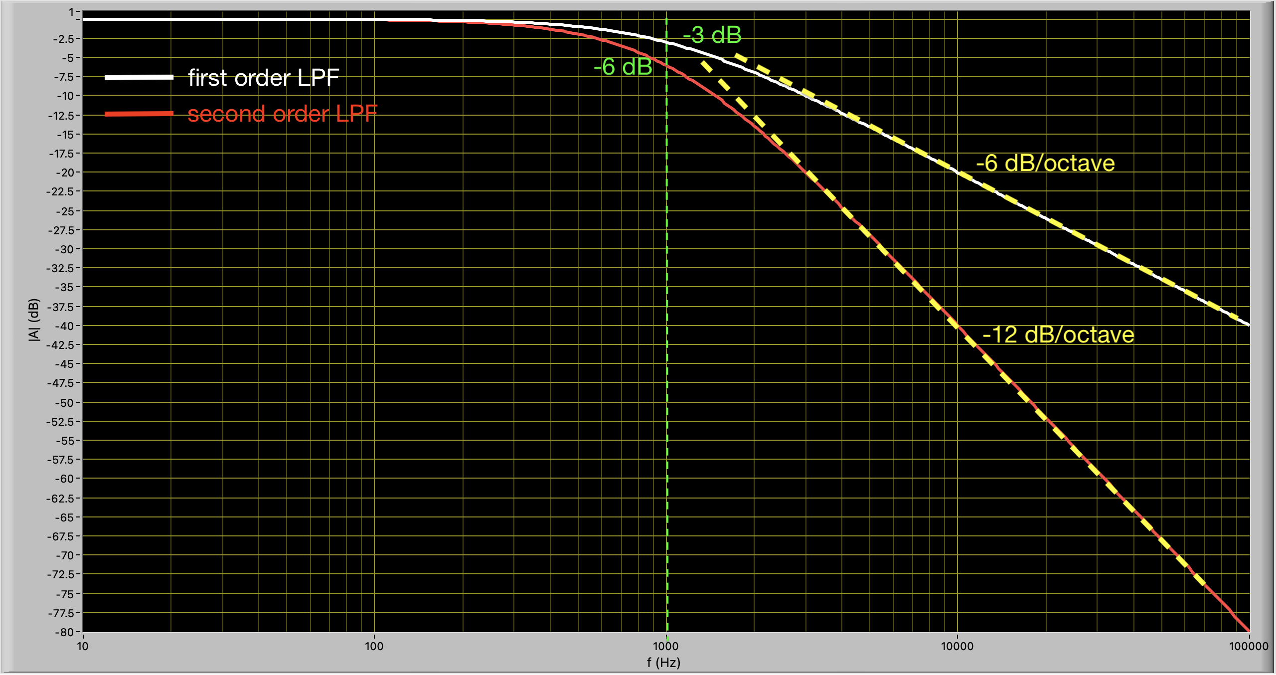
Fig. 50 Comparison of first and second order low-pass filter with 1 kHz cut-off frequency

To calculate the influence of the first filter on the second filter Thévenin is used to replace the first filter plus the input signal by a new input source \(V_{\rm Th}\), and a new output impedance \(Z_{\rm Th}\). Fig. 47 changes to Fig. 51.

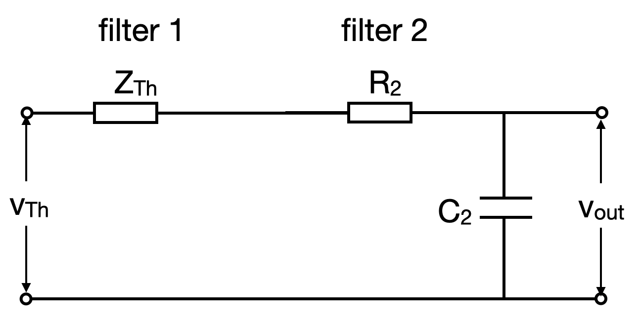
Fig. 51 Replacement circuit second order low-pass filter

The total transfer function is given by:

(56)\[ A(\omega)=\dfrac{1}{1+j\omega \tau(2+\alpha )-\omega^{2} \tau^{2}}, \]

where \(\alpha = R_{1}/R_{2}\).

Comparison of eqns. (52) and (56) shows that the load (the influence of the first filter) may be neglected when \( \alpha \) is very small. This is true when: \(R_{2} \gg R_{1}\). A far better design for this circuit is given in Fig. 52 with \(R_{2} = 10R_{1}\) and \(C_{2} = 0.1C_{1}\). So \(R_{1}C_{1} = R_{2}C_{2}\) is still true.

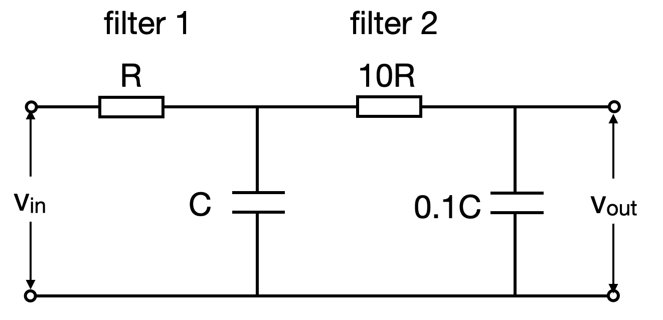
Fig. 52 Adapted second order low-pass filter

A similar reasoning can be held for a band-pass filter composed of a low and a high pass filter (Fig. 53)

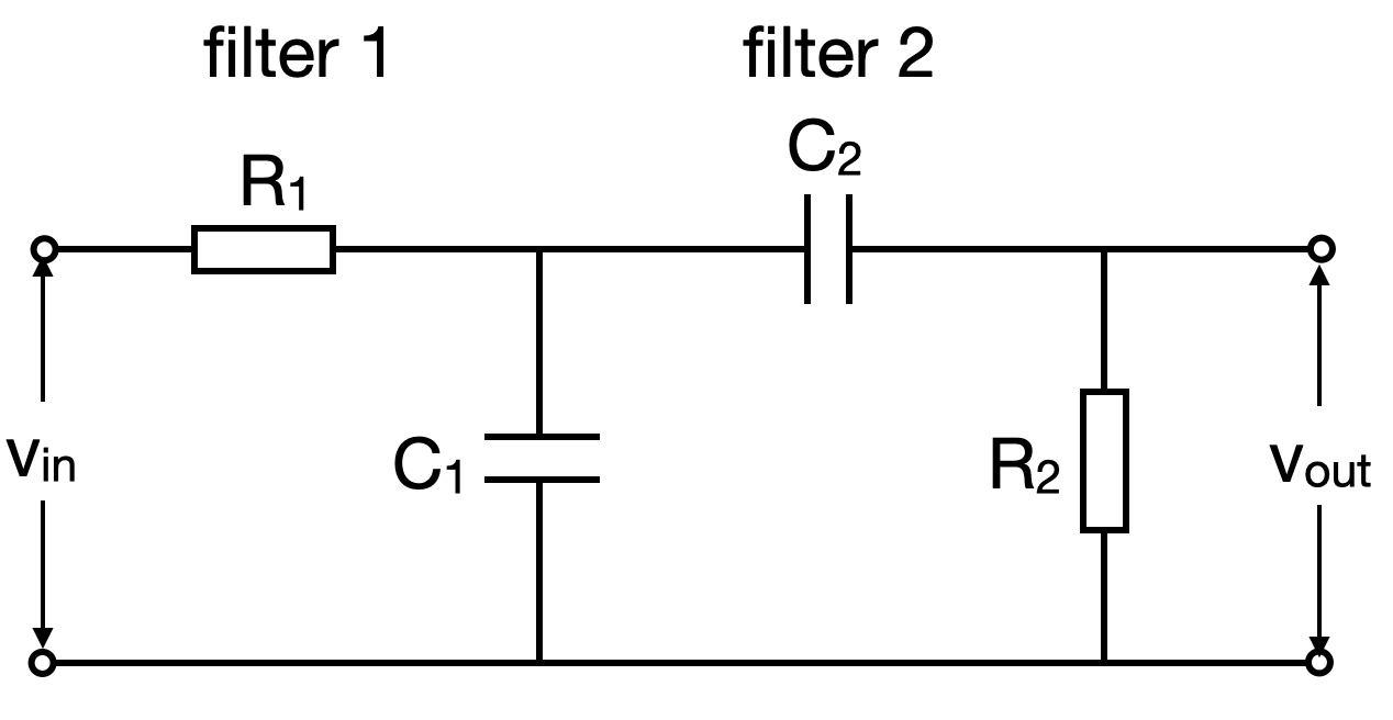
Fig. 53 Band-pass filter

When the load of the low-pass filter influences the high-pass filter, the transfer function of this band-pass filter is given by:

(57)\[ A(\omega)=\dfrac{j\omega \tau_{2}}{1+j\omega (\tau_{1}+\tau_{2}+\alpha \tau_{2})-\omega^{2}\tau_{1}\tau_{2}}, \]

where (also in this case) \(\alpha = R_{1}/R_{2}\).

Exercise 4.3

• Derive eqn. (57).

• Without weakening the signal that is passed through, which \( \tau \) must be the largest in this band-pass filter?

• For what value of \( \alpha \) is the effect of the load from first filter acting on the second filter the smallest?

• How many dB/octave and how many dB/decade does this filter drop for low and high frequency?

• Open Mult 4.3 and verify your results for different values of \( \alpha \). Keep the values of \(\tau_{1}\) and \(\tau_{2}\) constant each time.

Answer

• The Thévenin voltage for the LPF is given by

(58)\[ V_{\rm Th} = \frac{1}{1 + j \omega \tau_1} \cdot V_{\rm in }. \]

The Thévenin impedance for the LPF is given by

(59)\[ Z_{\rm Th} = (R_1 || C_1) = \left[ \frac{1}{R_1} + \frac{j \omega C_1}{1} \right]^{-1} = \left[ \frac{1 + j \omega R_1 C_1}{R_1} \right]^{-1} = \frac{R_1}{1 + j \omega \tau_1}. \]

The band filter circuit is shown in Fig. 54.

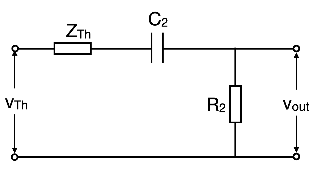
Fig. 54 Band filter circuit

The transfer function for this circuit is

(60)\[\begin{split} \begin{split} A' ( \omega ) &= \frac{R_2}{\left( Z_{\rm Th} + 1 / j \omega C_2 \right) + R_2} \\ &= \frac{R_2}{\left( R_1 / (1 + j \omega \tau_1) + 1 / j \omega C_2 \right) + R_2} \\ &= \frac{1}{\frac{R_1}{R_2} \left( 1 / (1 + j \omega \tau_1) \right) + 1 / j \omega \tau_2 + 1} \\ &= \frac{1}{\alpha / (1 + j \omega \tau_1) + 1 / j \omega \tau_2 + 1}. \end{split} \end{split}\]

The total transfer function is obtained by multiplying \(A' ( \omega )\) by \(V_{\rm Th}\):

(61)\[\begin{split} \begin{split} A ( \omega ) &= \frac{1}{1 + j \omega \tau_1} \cdot \frac{1}{\alpha /( 1 + j \omega \tau_1) + (1 / j \omega \tau_2 ) + 1} \\ &= \frac{1}{\alpha + \frac{1 + j \omega \tau_1}{j \omega \tau_2} + 1 + j \omega \tau_1} \\ &= \frac{j \omega \tau_2}{\alpha j \omega \tau_2 + 1 + j \omega \tau_1 + j \omega \tau_2 - \omega^2 \tau_1 \tau_2} \\ &= \frac{j \omega \tau_2}{1 + j \omega \left( \tau_1 + \tau_2 + \alpha \tau_2 \right) - \omega^2 \tau_1 \tau_2}. \end{split} \end{split}\]

The modulus \(\left| A (\omega) \right|\) is given by:

(62)\[\begin{split} \begin{split} \left| A ( \omega ) \right| &= \frac{\left| j \omega \tau_2 \right|}{\left| 1 + j \omega \left( \tau_1 + \tau_2 + \alpha \tau_2 \right) - \omega^2 \tau_1 \tau_2 \right|} \\ &= \frac{\omega \tau_2}{\sqrt{\left( 1 - \omega^2 \tau_1 \tau_2 \right)^2 + \omega ^2 \left( \tau_1 + \tau_2 + \alpha \tau_2\right)^2}} \\ &= \frac{\omega \tau_2}{\sqrt{1 - 2 \omega^2 \tau_1 \tau_2 + \omega^4 \tau_1^2 \tau_2^2 + \omega^2 \left( \tau_1^1 + \tau_2^2 + \alpha^2 \tau_2^2 + 2 \tau_1 \tau_2 + 2 \alpha \tau_1 \tau_2 + 2 \alpha \tau_2^2 \right)}} \\ &= \frac{\omega \tau_2}{\sqrt{1 + \omega^4 \tau_1^2 \tau_2^2 + \omega^2 \tau_1^2 + \omega^2 \tau_2^2 + \omega^2 \alpha^2 \tau_2^2 + 2 \omega^2 \alpha \tau_1 \tau_2 + 2 \omega^2 \alpha \tau_2^2}} \\ &= \frac{\omega \tau_2}{\sqrt{1 + \omega^2 \left(\omega^2 \tau_1^2 \tau_2^2 + \tau_1^2 + \tau_2^2 + \alpha^2 \tau_2^2 + 2 \alpha \tau_1 \tau_2 + 2 \alpha \tau_2^2 \right)}}. \end{split} \end{split}\]

• We can determine which \(\tau\) must be the largest in the band pass filter: when the signal passed through cannot be weakened. Based on the cut-off value of \(1 / \tau\), we can determine which \(\tau\) must be largest:

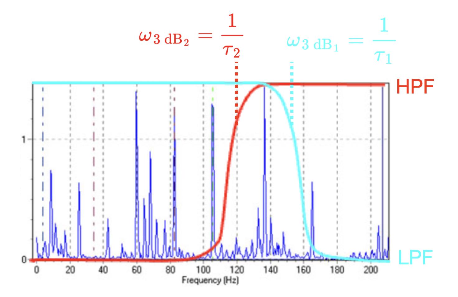
Fig. 55 Band filter with LPF and HPF sketch

The cut-off value of the first filter needs to be high which means \(\tau_1\) needs to be low. Therefore, \(\tau_2 > \tau_1\).

• From (57) it follows that when \(\alpha = \frac{R_1}{R_2}\) is small the effect of the load of the first filter acting on the second filter is minimal (the nominator \(j \omega \tau_2\) is an additional factor due to the presence of the first filter but this contribution is constant). This is the case when \(R_2 \gg R_1\).

• For large frequencies eq. (62) may be approximated by

(63)\[ |A( \omega ) = \frac{\omega \tau_2}{\sqrt{1 + \omega^2 \left(\omega^2 \tau_1^2 \tau_2^2 + \tau_1^2 + \tau_2^2 + \alpha^2 \tau_2^2 + 2 \alpha \tau_1 \tau_2 + 2 \alpha \tau_2^2 \right)}} \approx \frac{\omega \tau_2}{\omega \cdot \omega \tau_1 \tau_2} = \frac{1}{\omega \tau_1}. \]

The filter then drops

(64)\[ \frac{|A( \omega_2)|}{|A( \omega_1)|} = \frac{\omega_1 \tau_1}{\omega_2 \tau_2} = \frac{\omega_1 \tau_1}{2 \omega_1 \tau_1} = \frac{1}{2} \]

per octave. So we get \(20 \log_{10}(\frac{1}{2}) = - 6\) dB/octave, or

(65)\[ \frac{|A( \omega_2)|}{|A( \omega_1)|} = \frac{\omega_1 \tau_1}{\omega_2 \tau_2} = \frac{\omega_1 \tau_1}{10 \omega_1 \tau_1} = \frac{1}{10} \]

per decade. So we get \(20 \log_{10}(\frac{1}{10}) = - 20\) dB/decade.

• For low frequencies eq. (62) may be approximated by

(66)\[ |A( \omega ) = \frac{\omega \tau_2}{\sqrt{1 + \omega^2 \left(\omega^2 \tau_1^2 \tau_2^2 + \tau_1^2 + \tau_2^2 + \alpha^2 \tau_2^2 + 2 \alpha \tau_1 \tau_2 + 2 \alpha \tau_2^2 \right)}} \approx \frac{\omega \tau_2}{1} = \omega \tau_2. \]

The filter then drops

(67)\[ \frac{|A( \omega_2)|}{|A( \omega_1)|} = \frac{\omega_2 \tau_2}{\omega_1 \tau_2} = \frac{2 \omega_1 \tau_2}{\omega_1 \tau_2} = 2 \]

per octave. So we get \(20 \log_{10}(2) = +6\) dB/octave, or

(68)\[ \frac{|A( \omega_2)|}{|A( \omega_1)|} = \frac{\omega_2 \tau_2}{\omega_1 \tau_2} = \frac{10 \omega_1 \tau_2}{\omega_1 \tau_2} = 10 \]

per decade. So we get \(20 \log_{10}(10) = +20\) dB/decade.

The behavior of this filter has been investigated using Multisim for three different values of \(\alpha\):

• \(\alpha = 0.01\) (\(R_1 = 10 \; \Omega, \; C_1 = 5000 \; {\rm nF}, \; R_2 = 1000 \; \Omega\) and \(C_2 = \; 1 \; \mu {\rm F}\))

• \(\alpha = 1\) (\(R_1 = 1000 \; \Omega, \; C_1 = 50 \; {\rm nF}, \; R_2 = 1000 \; \Omega\) and \(C_2 = \; 1 \; \mu {\rm F}\))

• \(\alpha = 100\) (\(R_1 = 1000 \; \Omega, \; C_1 = 50 \; {\rm nF}, \; R_2 = 10 \; \Omega\) and \(C_2 = \; 100 \; \mu {\rm F}\))

The results are shown in Fig. 56 to Fig. 58.

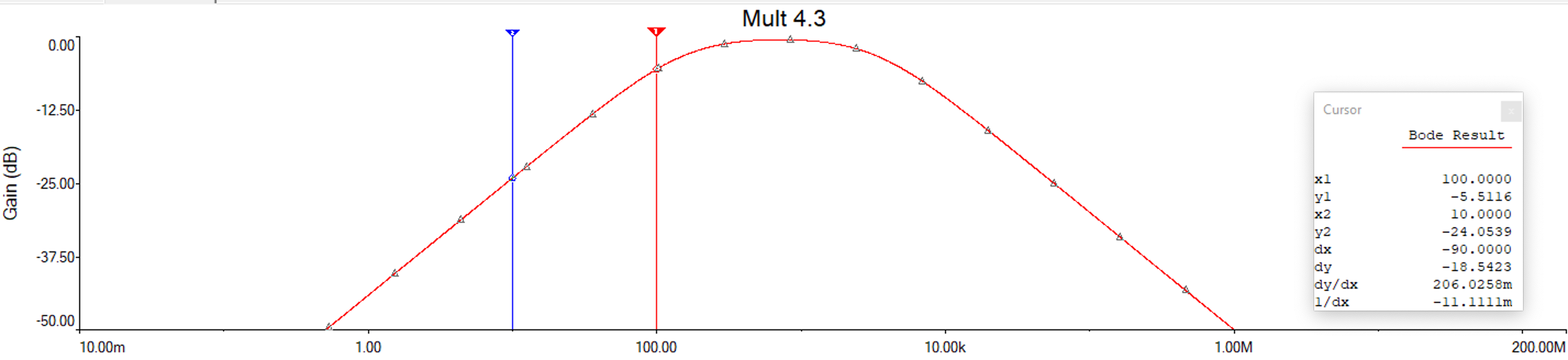
Fig. 56 \(\alpha = 0.01\). Note that the filter drops with 20 dB/decade.

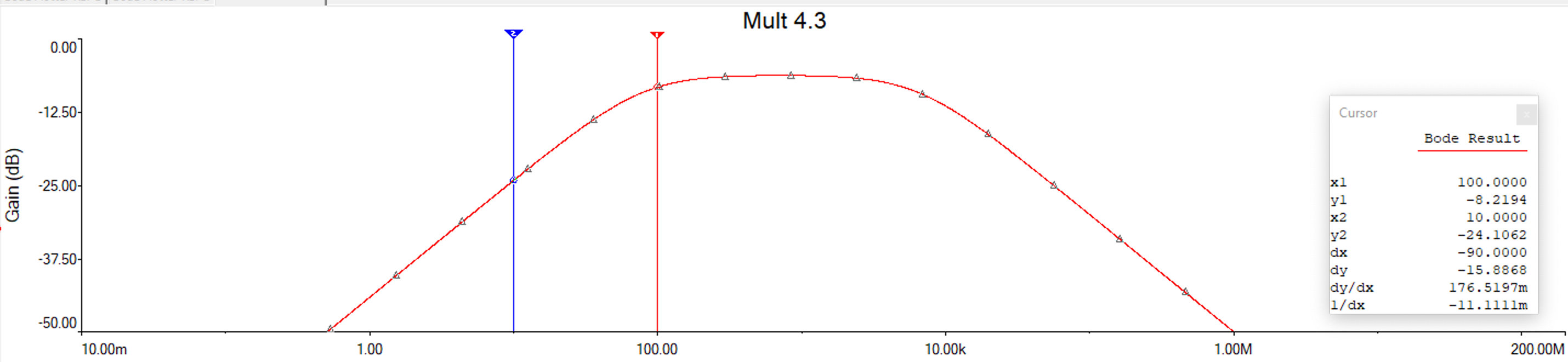
Fig. 57 \(\alpha = 1\). The band becomes wider as compared to \(\alpha = 0.01\) and the signal gets slightly attenuated.

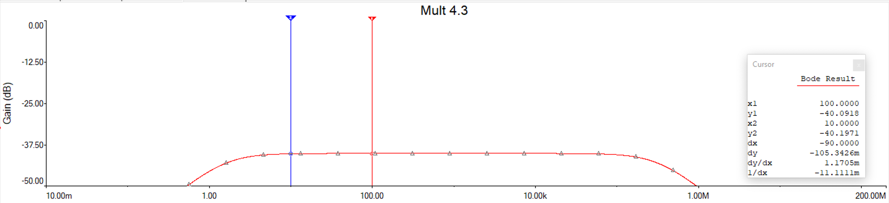
Fig. 58 \(\alpha = 100\). The band becomes very wide and the signal is strongly attenuated.

Resonance circuits

An ideal band filter is a filter that passes through a signal for a small frequency range, and filters out frequencies above and below this band pass as much as possible. This means that for such a filter the amplitude function needs to have a very steep fall for the low and high frequencies. As Assignment 4.3 shows this is certainly not the case for the band filter shown in Fig. 53. A much better result can be obtained by using a combination of \(R\), \(L\) and \(C\).
Fig. 59 shows a parallel \(LC\)-circuit which can be used as a band filter.

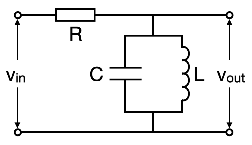
Fig. 59 Parallel \(LC\)-circuit

The transfer function is given by:

(69)\[ A(\omega)=\dfrac{\left( Z_{C} \parallel Z_{L} \right)}{R + \left( Z_{C} \parallel Z_{L} \right)}=\dfrac{j\omega L}{R(1-\omega^{2} LC )+j\omega L} \]

The frequency \( \omega_{0} \), for which \( |A(\omega)| \) is maximal, is called the resonant frequency of the filter. It is easy to see that \( \omega_{0}=\frac{1}{\sqrt{LC}} \). In that case \( Z_{C}\parallel Z_{L}=\infty \). Substitution into eqn. (69) yields \( |A(\omega_{0})|=1 \). In that case \(|A(\omega)|\) is real. For both \( \omega \ll \omega_{0} \) and \( \omega \gg \omega_{0} \) the amplitude function is \( |A(\omega)|\Rightarrow 0 \).
The extent to which this band filter is very steep depends on the values of \(R\), \(L\) and \(C\). A common standard used for this purpose is the quality factor Q, which is defined as:

(70)\[ Q=\dfrac{\omega_{0}}{\Delta \omega }, \]

where \( \Delta \omega \) is the bandwidth of the filter. \( \Delta \omega \) is equal to the distance between the two 3 dB points. The 3 dB points can still be found using (43):

(71)\[ \dfrac{|A(\omega_{3 {\rm dB}})|}{|A|_{\rm max}}=\dfrac{1}{\sqrt{2}}. \]

From eqn. (69) it follows that:

(72)\[ |A(\omega)|=\dfrac{1}{\sqrt{1+R^{2}\left(\omega C-\dfrac{1}{\omega L}\right)^{2}}} \]

Combination of eqns. (71) and eqn. (72) gives:

(73)\[\begin{split} \begin{split} R^{2}\left(\omega C-\dfrac{1}{\omega L}\right)^{2} &= 1 \\ \Rightarrow R\left(\omega C-\dfrac{1}{\omega L}\right) &= \pm 1 \\ R(\omega^{2}LC-1) &= \pm \omega L \end{split} \end{split}\]

Further elaboration of eqn. (73), which takes account of the fact that \( \omega \geqq 0 \), yields

(74)\[ \nonumber \left.\begin{aligned} \omega_{3dB}&=\dfrac{-L+\sqrt{L^{2}+4R^{2}LC}}{2RLC}\ \omega_{3dB}&=\dfrac{L+\sqrt{L^{2}+4R^{2}LC}}{2RLC} \end{aligned} \right\} \]

(75)\[ \Rightarrow \Delta \omega = \dfrac{1}{RC} \]

Using \( \omega_{0}=\dfrac{1}{\sqrt{LC}}\) and eqn. (75) the quality factor \(Q\) (eqn. (70)) yields:

(76)\[ Q=R\sqrt{\dfrac{C}{L}} \]

Lab exercises

Note

In the following exercises a Bode plot need to be measured. This always means both a plot of the amplitude of the transfer function and a plot of the phase transfer function.

Exercise 4.4

• Design in Multisim a low-pass filter as shown in Fig. 42 with a -3 dB point of 1 kHz and make a Bode plot of the transfer function.

• Build this filter with NI Elvis.

• Determine the -3 dB point from the Bode plot.

• Compare the experimentally determined values with the results of the simulation. Plot for this the data sets of both amplitude transfer functions in one graph and both phase transfer function in one graph.

Note

The measured data in the Bode Analyzer of NI Elvis is saved with the ‘Log’ button (Lower right corner). Save the data using a dB-scale.
The simulation data in Multisim is saved in the ‘Grapher’ with the ‘Export to Excel’ button (Upper right corner). The ‘Grapher’ is found in the View-menu of Multisim. The red arrow on the left side of the graph indicates which graph is saved. Selecting is done by a click on the graph. Multisim always saves the data using a linear scale so you will need to convert the modulus to dB scale for comparison with the experimental data.

Exercise 4.5

• Design in Multisim a band-pass filter as shown in Fig. 53 having the following properties

  • \( \omega_{3 \, {\rm dB}} \) at the lower end is located at \(f = 200 \, {\rm Hz}\).

  • \( \omega_{3 \, {\rm dB}} \) on the high side is at \(f = 20 \, {\rm kHz}\).

  • \(|A|_{\rm max} > 0.9\).
    So the influence of the first filter on the second filter is minimal!

• First show the transfer function of this filter in a Bode plot with the aid of Multisim.

• Build this filter.

• Determine the -3 dB point from the measured Bode plot.

• Plot the simulation and the measured data in one graph and compare the experimentally determined values with the results of the simulation. Values like \( \omega_{3 \, {\rm dB}} \) at the low and high side and \(|A|_{\rm max}\).

Exercise 4.6

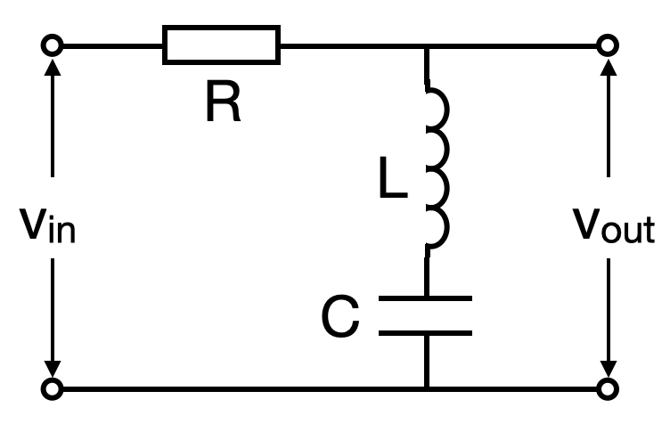
Fig. 60 Serie \(LC\)-circuit

• Determine the complex transfer, amplitude and phase function for the circuit in Fig. 60.

• Investigate the behaviour of the circuit.

• What is the use of this circuit?

• Derive an expression for the quality factor \(Q\) and the resonance frequency \( \omega_{0} \).

• Design in Multisim a circuit with a resonant frequency of \(1 \, {\rm kHz}\) and try to maximize the \(Q\) factor.

• Make a Bode plot.

• Verify your results with the calculated \(Q\) and \( \omega_{0} \) values.

• Build this filter.

• Measure a Bode plot with NI Elvis.

• Verify your results with the results of the simulation. Plot again the data in one graph. Give an explanation for any differences.